Here’s some knowledge gathered during my internships.
RNA (or ribonucleic acid) is a macromolecule that has a number of biological functions such as:
- being the intermediary support of genetic information between DNA and proteins
- being the catalyst of the peptidyl-transferase action leading to the creation of a peptidic bond (protein synthesis)
- being a regulator of genetic expression through riboswitchs or small interfering molecules
- being an inactivator of chromosomes through long interfering molecules
If sequence conservation is crucial for proteins, this central dogma is put under questioning for RNAs. Indeed, it seems that secondary and tertiary structure conservation are more relevant for RNAs.
The 3D structure of an RNA is the set of coordinates of its atoms in space. This kind of data can be found in PDB files, then using PyMOL (The PyMOL Molecular Graphics System, Schriödinger, LLC, 2010) one can represent the structure of the RNA (see Figure - 3FU2).
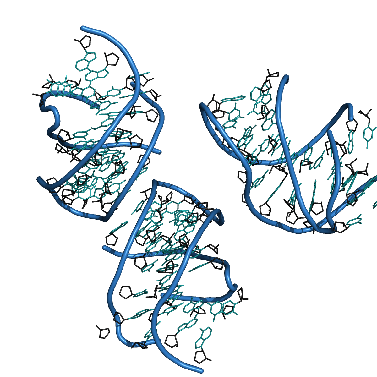
Figure - 3FU2
3D structure of RNA 3fu2 obtained using PyMOL on a PDB file.
Here, we will focus on the secondary structure of RNAs.
How to represent RNA structures?
Before everything else (even defining properly what is a secondary structure), let’s take a quick tour of the way RNAs are represented: they are several types of representation and each of them has limits.
The squiggle-plot representation (and common interest patterns)
The squiggle-plot representation is the closest to what we may draw manually and “naturally” to represent an RNA. It is the representation that allows the best comprehension of what happens in the structure, as you can see in the next 4 pictures. Those pictures represent the most common interest patterns in RNA.
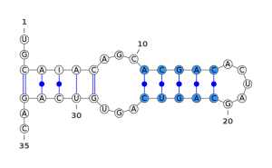
Figure - RNA stem
In blue, a stem structure. A stem is a structure of double stranded RNA creating a series of consecutive basepairs.
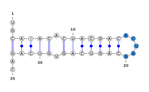
Figure - RNA hairpin
In blue, a hairpin structure. A hairpin loop is the simplest kind of loop we can obtain in an RNA. It is located at the end of a stem.
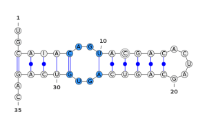
Figure - RNA interior loop
In blue, an interior loop. An interior loop is a structure consisting in a set of unpaired bases flanked by two stems.
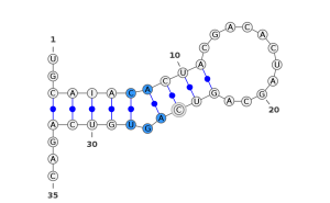
Figure - RNA bulge
In blue, a bulge. A bulge is a structure that occurs when there are some unpaired bases on one side of the stem.
However, this representation is not well suited for structure alignment, as explain in a review of Schirmer et al. (Introduction to RNA secondary structure comparison, Schirmer Stefanie et al., Humana Press, 2014).
Moreover, those drawings are produced by algorithms whose main purpose are pretty-printing and overlapping avoindance which is far from reality.
The dot-parenthesis representation
The dot-parenthesis representation (or dps) it of this kind:
00 01 02 03 04 05 06 07 08 09 10
 G  C  A  A  U  G  C  U  U  A  A
 .  .  (  (  .   . .  )  )  .  .
Bases (02, 08) interact, as well as bases (03, 07).
This kind of representation is used by VARNA (VARNA: Interactive drawing and editing of the RNA secondary structure, Darty et al. Bioinformatics, 2009). It is a nice tradeof between practicity and readability.
The tree representation
In fact, a dps is a tree.
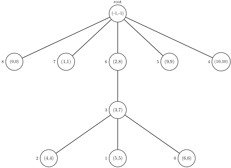
Figure - Tree reprensentation of RNA
A tree representation of RNA secondary structure ..((...))..
I guess you see how it works? If you’re not convinced, here’s the algorithm written in c++:
Tree< std::vector<int> >* dps::parse(int & index)
{
    /* Start point of the recursion */
    int start = index;

    /* Create a tree */
    Tree< std::vector<int> >* current_root = new Tree< std::vector<int> >();

    /* Traversal, character by character of the sequence */
    while (index < (int)this->sequence.length())
    {
        index ++;
        switch (this->sequence[index -1])
        {
            case '.':
            {
                /* It's a leaf */
                std::vector<int> pos = { index - 1, index - 1 };
                Tree< std::vector<int> >* leaf = new Tree< std::vector<int> >(pos);
                current_root->append_child(leaf);
                break;
            }
            case '(':
            {
                 /* Recursive call to find the whole tree */
                 Tree< std::vector<int> >* node = parse(index);
                 current_root->append_child(node);
                 break;
            }
            case ')':
            {
                 /* All children are discovered, return the subtree */
                 std::vector<int> current_pos = { start - 1, index - 1};
                 current_root->set_position(current_pos);
                 return current_root;
                 break;
             }

             default:
             {
                 /* This should not happen */
                 std::stringstream stream;
                 stream << "Sequence has an unexpected character that isn't ( . or )\n";
                 DPSInvalidInput myerror(stream.str());
                 throw myerror;
                 break;
              }
        }
}
The tag of the tree is a vector of positions:
- For a leaf, the position of the
., twice. - For an internal node, the position is the tuple given by the position of the
(and its matching).
In Figure - Tree reprensentation of RNA, the root has a tag (-1, -1) because it is virtual, it does not match any biological reality.
This root is virtual because the first character in the dps is a . and therefore a leaf, which implies we obtain a forest (family of trees) and we need to root it.
What is an RNA secondary structure?
Definitions
The structure of RNA is the result of the pairing of bases thanks to hydrogen bonds. We will call those bonds “arcs” and the given structure an “arc-annotated sequence”.
Let two ( (i_1, i_2) ) and ( (i_3, i_4) ) be two arcs of an RNA. They are said to be independant if and only if they abide by one of the following inequalities: $$i_1 \lt i_2 \lt i_3 \lt i_4 \text{ or } i_3 \lt i_4 \lt i_1 \lt i_2$$ They are said to be nested if and only if they abide by one of the following inequalities: $$i_1 \lt i_3 \lt i_4 \lt i_2 \text{ or } i_3 \lt i_1 \lt i_2 \lt i_4$$
With those definitions, we are equiped to define an RNA secondary structure:
The secondary structure of an RNA is the largest subsets of nested and independant arcs that may be extracted from an arc-annotated RNA structure.
Planarization of RNA structures
So, basically, we’re going to need to take out some arcs from the arc-annotated sequence in order to get a dps. Taking out arcs, e.g. interactions, is a problem called RNA planarization which requires some new definitions.
A generic structure is a graph \((V, A)\), where \(V = [|1;n|]\) where \(n\) is the length of the RNA structure and $$A \subseteq {(i, j) \in [|1;n|]^2 | i < j }$$
A generic structure \(S = (V, A)\) is included in a generic structure \(S'' = (V, A'') \) if and only if \( A \subseteq A''\).
Now we can define the planarization problem:
Planarization problem of RNAs From a generic structure \(S = (V, A)\), return a generic structure \(S' = (V, A')\) that respects:
- inclusivity \(S \subseteq S' \)
- planarity $$ \forall (i, j) \neq (i', j') \in A', (i \neq i') \wedge (j \neq j') \wedge \left( [| i; j |] \cap [| i'; j'|] = \begin{cases} \emptyset \\ [| i; j |] \\ [| i';j' |] \end{cases} \right) $$
- optimality \(\forall A'' \subseteq A \) such as \((V, A'')\) planar, \(|A''| \leq |A'|\)
How do you find a solution to this problem? The idea is that every structure can be break down the way explained in the picture bellow:
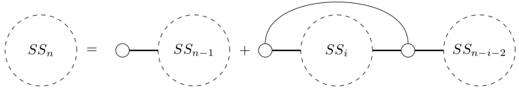
Figure - Decomposition of structures
Decomposition of a super structure of size \(n\): either a super structure of size \(n - 1\) and an unpaired base or a structure of size \(i\) nested in an arc and a structure of size \(n-i-2\)
I’m not gonna give you the algorithm for this problem (yet). Below is an example of planarization of an arc-annotated structure:
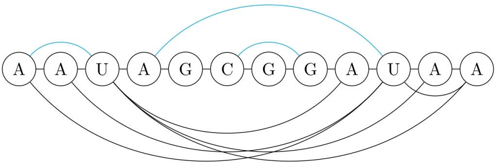
Figure - Decomposition example
An example of planarization. In blue the arcs preserved by the planarization, in black the arcs removed by the planarization.
That’s it for today!